How do we characterize 2D materials?
Making thin sheets is only the beginning. How much material did we collect? How thin is it? Did its structure survive? Follow six measurement methods from the first question to the evidence.
What do we need to know about a 2D material?
A 2D material is made of extremely thin sheets: a single layer, or a small stack of layers, of atoms. Separating these layers from a thicker crystal is called exfoliation. But after making the material, how do we know what we have?
We need to measure it. How wide are the sheets? How thick? Have their atoms kept the same bonds and arrangement? Characterization means answering these questions. Metrology is the science of measurement: checking our instruments, choosing samples that fairly represent the material, and understanding how precise our answers are.
No single instrument answers everything. In this guide, each method adds one piece of evidence. I explain the idea first, then show results from my thesis on graphene, hexagonal boron nitride (h-BN) and molybdenum disulfide (MoS₂), where available.
One sample. Six questions.
Imagine a bottle of liquid containing tiny flakes. Scientists call this a dispersion. A darker bottle might contain more material, but appearance alone cannot tell us whether the flakes are thin, thick, clumped together or damaged.
Our story starts with how much material is in the liquid. We then look at the sheets, measure their height, examine the wider surface, and check their chemistry and atomic vibrations. You can follow the story in order or jump to a question below. In the lab, the order depends on the sample.
UV–Vis spectrophotometer
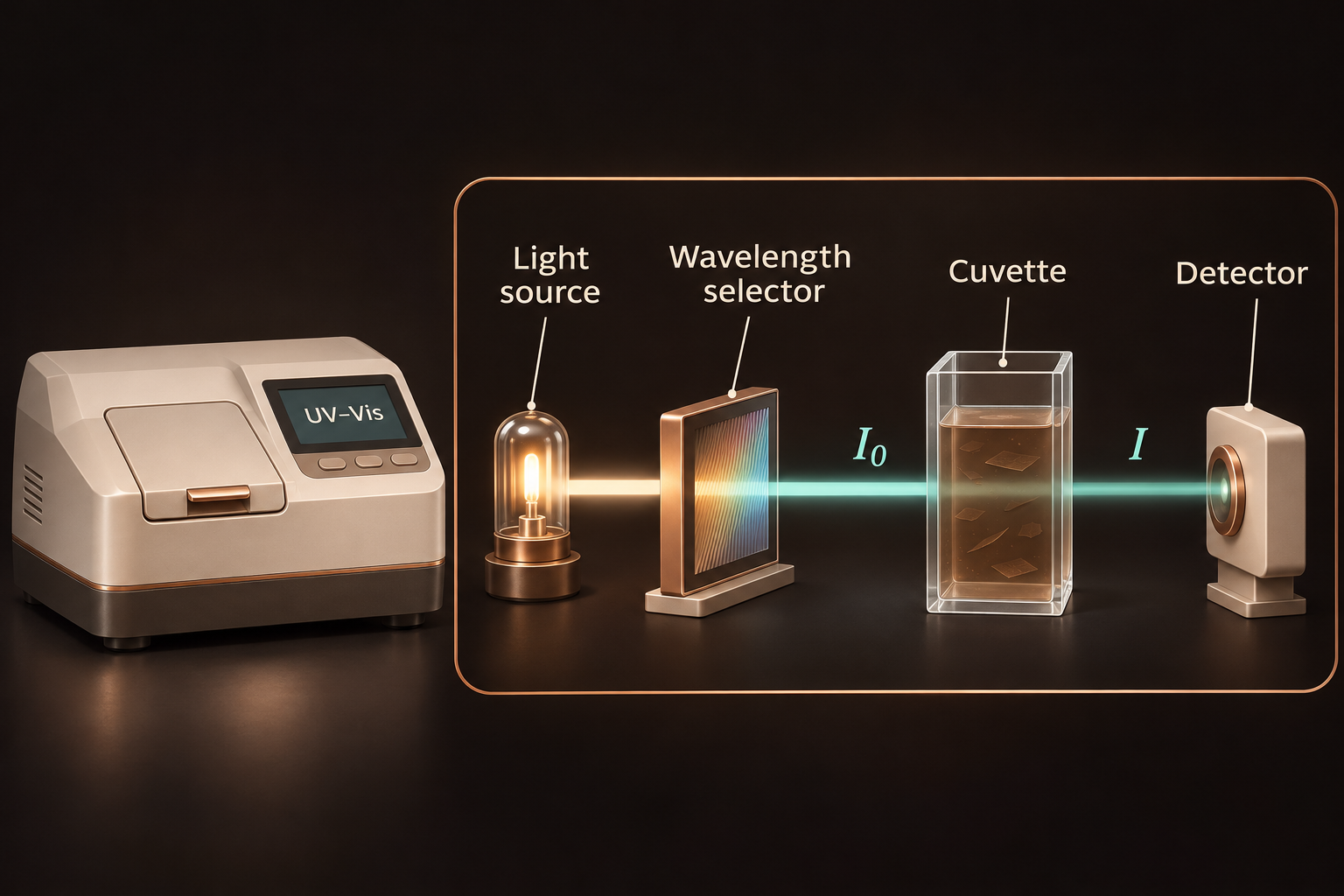
Before comparing two batches, we need to know how much solid each contains. UV–Vis, short for ultraviolet–visible, measures how light passes through the liquid. With a suitable reference measurement, it gives a quick estimate of concentration: the mass of solid in a given volume of liquid.
My thesis results
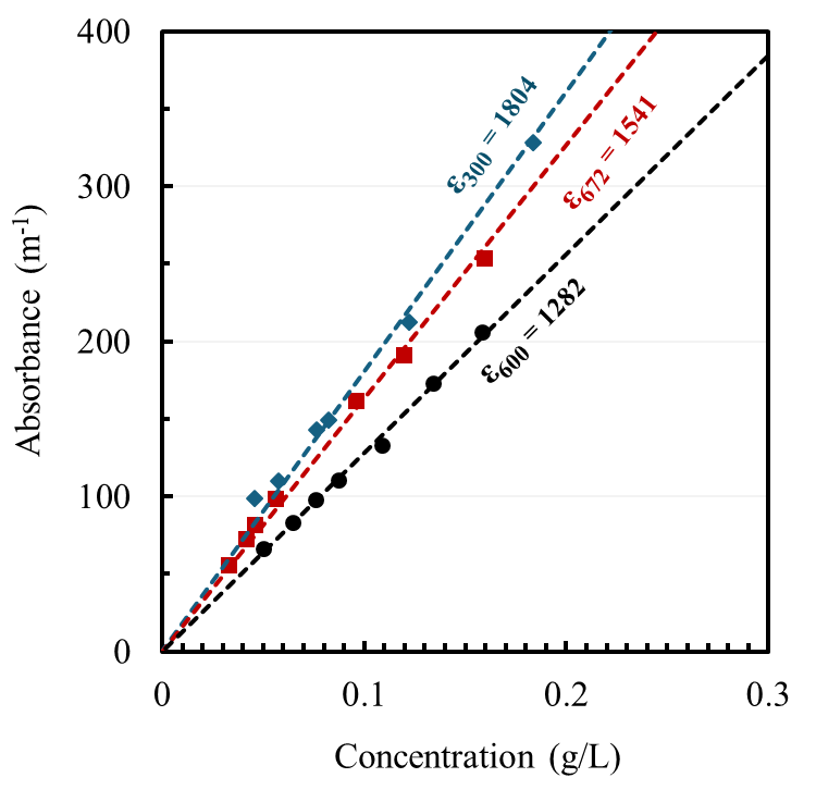
I first dried a known volume of each dispersion and weighed the solid left behind. This gave a concentration I could use as a reference. I then diluted the liquid by known amounts and measured how much light passed through each sample.
That comparison is called calibration: connecting an instrument reading to a known quantity. Each material needed its own calibration. The curves below show how I linked the optical signal to concentration.
Concentration tells us how much solid is in each litre. To find the total collected mass, we also need the liquid volume. To calculate the fraction recovered, we compare that mass with the amount of starting material. None of these numbers, by itself, tells us how many sheets are a single atomic layer.
Go deeper: measurements and scientific details
The calibrated Beer–Lambert form is A = αcl: A = log₁₀(I₀/I) is the blank-corrected optical attenuation, α the mass extinction coefficient at the chosen wavelength, c the mass concentration and l the optical path length. In a nanosheet dispersion, this apparent absorbance includes absorption and light scattered out of the detected beam. Use consistent units and the validated linear calibration range, then correct for dilution.
Calibration wavelengths: 300 nm for h-BN, 600 nm for graphene and 672 nm for MoS₂. The dry-mass measurement assumes that any other residue left after drying has been accounted for. It measures total recovered solids, not a separately measured single-layer or few-layer portion.
TEM, STEM and HRTEM
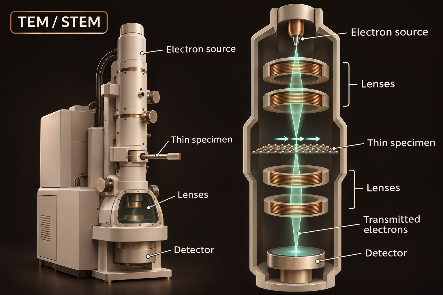
Knowing how much solid we collected does not tell us its shape. Did we separate broad sheets, or mostly make small chunks? Electron microscopes let us see individual flakes and, at higher resolution, examine the repeating arrangement of atoms in small regions.
My thesis results
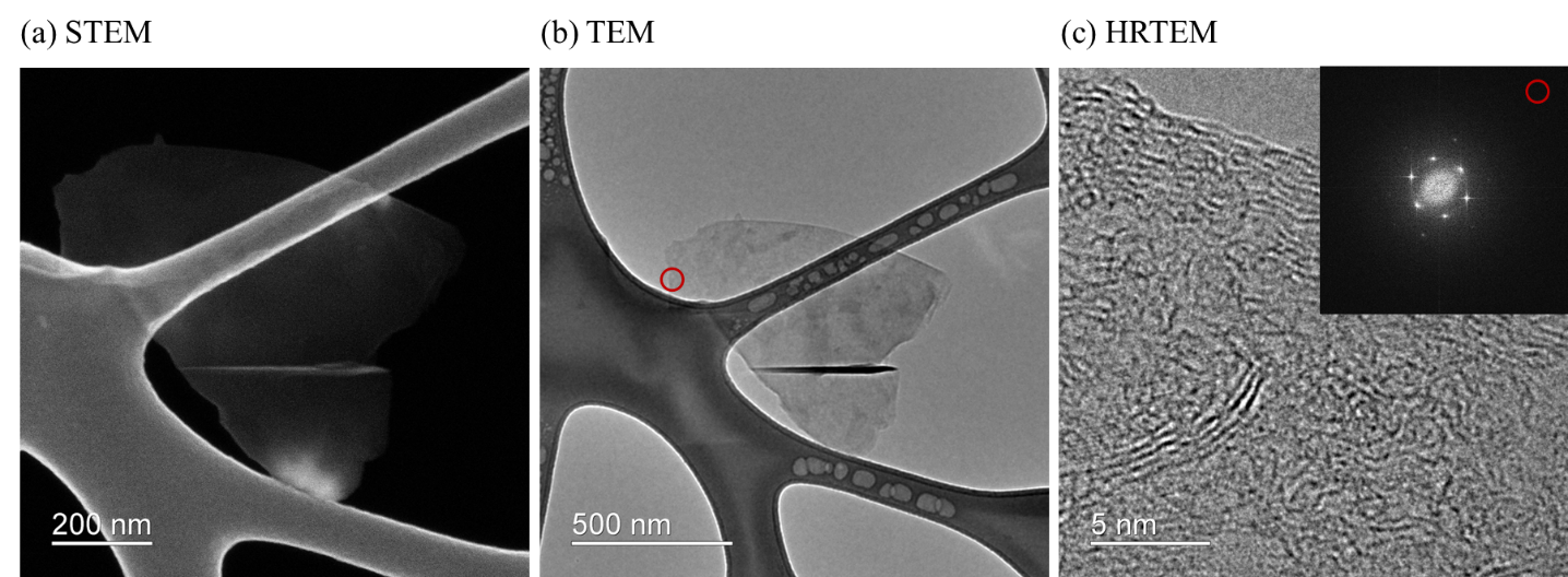
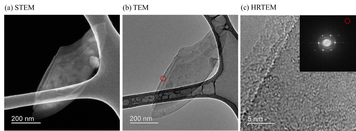
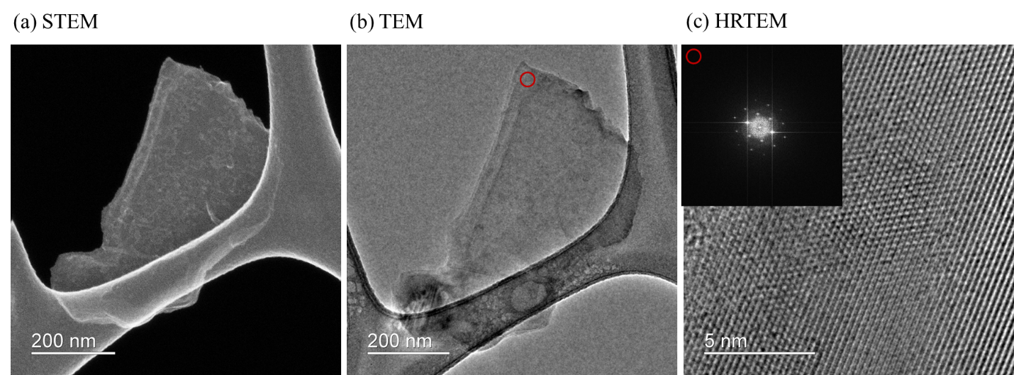
The graphene images showed broad sheets with folds and wrinkles. The h-BN sheets looked more elongated, while MoS₂ appeared as compact, plate-like flakes. The higher-resolution images also showed repeating atomic structure in small regions of all three materials.
For scale, a circle with the same area as one selected graphene flake would be about 717 nanometres across—less than one thousandth of a millimetre.
These images show that sheets are present. They do not tell us the typical size of every flake in the bottle. That would require measuring many flakes from different parts of the sample. Seeing ordered atoms in one region also does not prove that every sheet is free of defects.
Go deeper: measurements and scientific details
For selected flakes, the projected area—the area seen in the image—was approximately 0.404 µm² for graphene and 0.234 µm² for MoS₂. A circle with the same area as the selected graphene flake would be about 717 nm across. The selected h-BN flake had an aspect ratio of 2.84, meaning it was about 2.84 times as long as it was wide. These are individual examples, not averages of the whole batch.
HRTEM image contrast can reveal local lattice features. A fast Fourier transform (FFT) is a mathematical analysis of repeating patterns in an image; it is different from a separately recorded electron-diffraction pattern. Both can help investigate local atomic order.
Atomic force microscope (AFM)
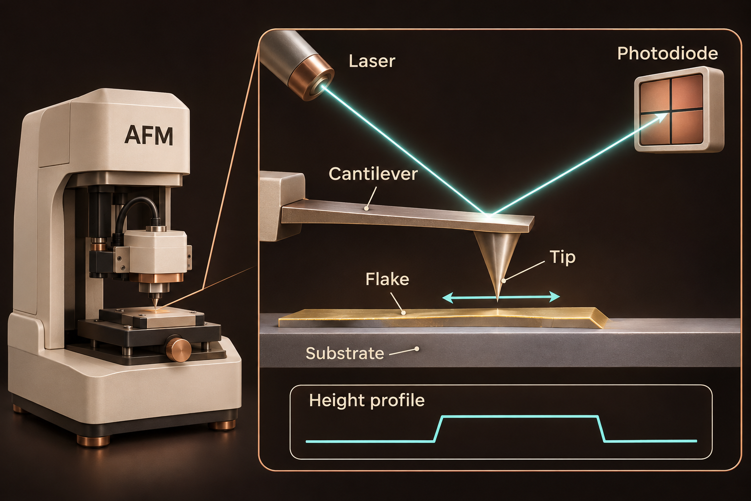
A wide flake can still be a thick stack. An atomic force microscope adds the missing height measurement. It follows the surface of a flake placed on a flat support, helping us work out how thin the flake is.
No original thesis result is presented here for this method.
Scanning electron microscope (SEM)
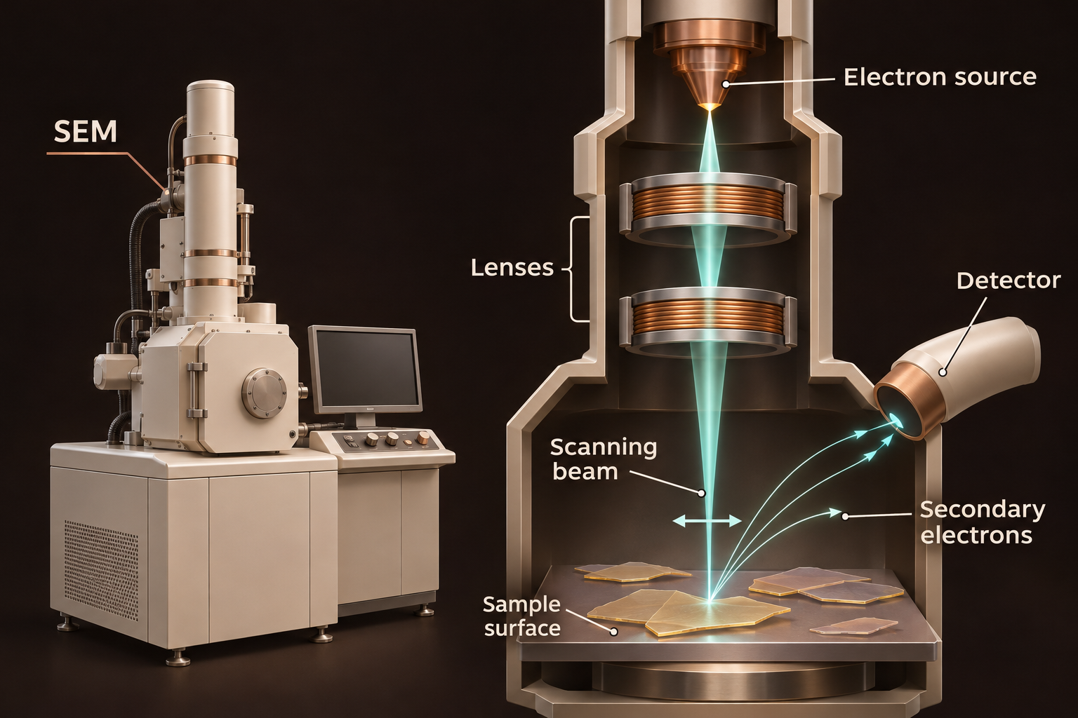
Now step back from a single flake. Are the sheets spread across a surface or gathered in clumps? A scanning electron microscope helps us explore these patterns and compare starting powders with the material left after processing.
No original thesis result is presented here for this method.
X-ray photoelectron spectrometer (XPS)
A sheet can keep its shape while its surface chemistry changes. Have new bonds formed, perhaps involving oxygen? X-ray photoelectron spectroscopy helps identify which elements are near the surface and how they are chemically bonded.
My thesis results
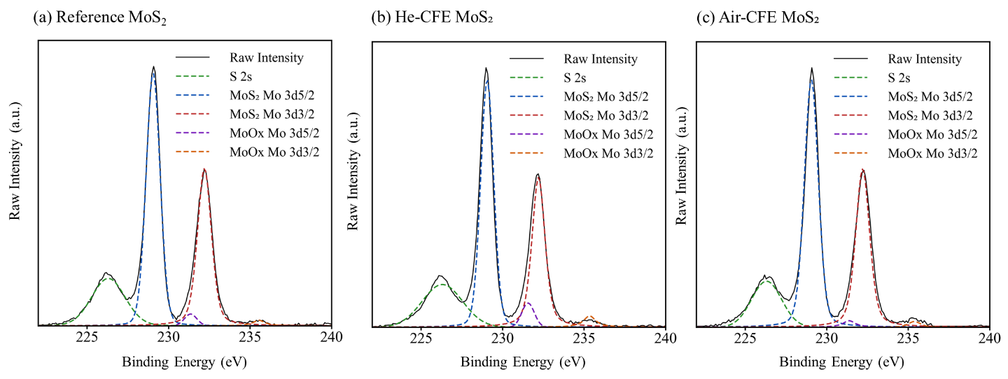
The strongest signals still matched the main bonding patterns of the starting materials. In other words, the surfaces largely kept their original chemical identity after processing.
There were smaller changes too. h-BN processed with air showed stronger oxygen-related signals than h-BN processed with helium. Graphene also showed some changes associated with edges and oxygen. MoS₂ showed small oxide-related signals, but air did not consistently give the largest change.
We cannot blame all of the oxygen signal on the gas used during processing. Newly exposed edges can also react while the material is collected in liquid, dried or stored. XPS measures the surface as it is when we test it, including that history.
Go deeper: measurements and scientific details
The fitted spectra were dominated by graphitic carbon for graphene, B–N bonding for h-BN, and Mo–S and sulfide signals for MoS₂. These assignments describe the main chemical environments near the surface, not long-range crystal order.
For MoS₂, no clear extra pair of lower-binding-energy Mo peaks associated with the 1T structure was resolved. This supported a mainly 2H product—the usual semiconducting structure—within the sensitivity of the measurement and the limits of peak fitting. It does not rule out a small undetected contribution from another structure.
Raman spectrometer
We have examined the shape and surface chemistry. Now we ask how the atoms vibrate. Raman spectroscopy measures a pattern of vibrations that helps identify the material and can reveal changes associated with thinning, edges or damage.
My thesis results
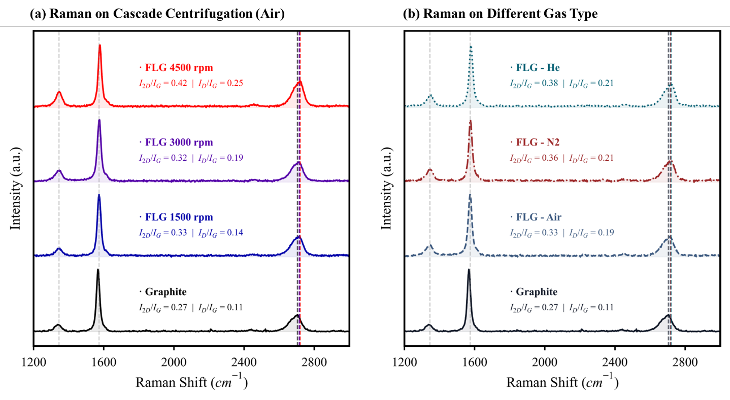
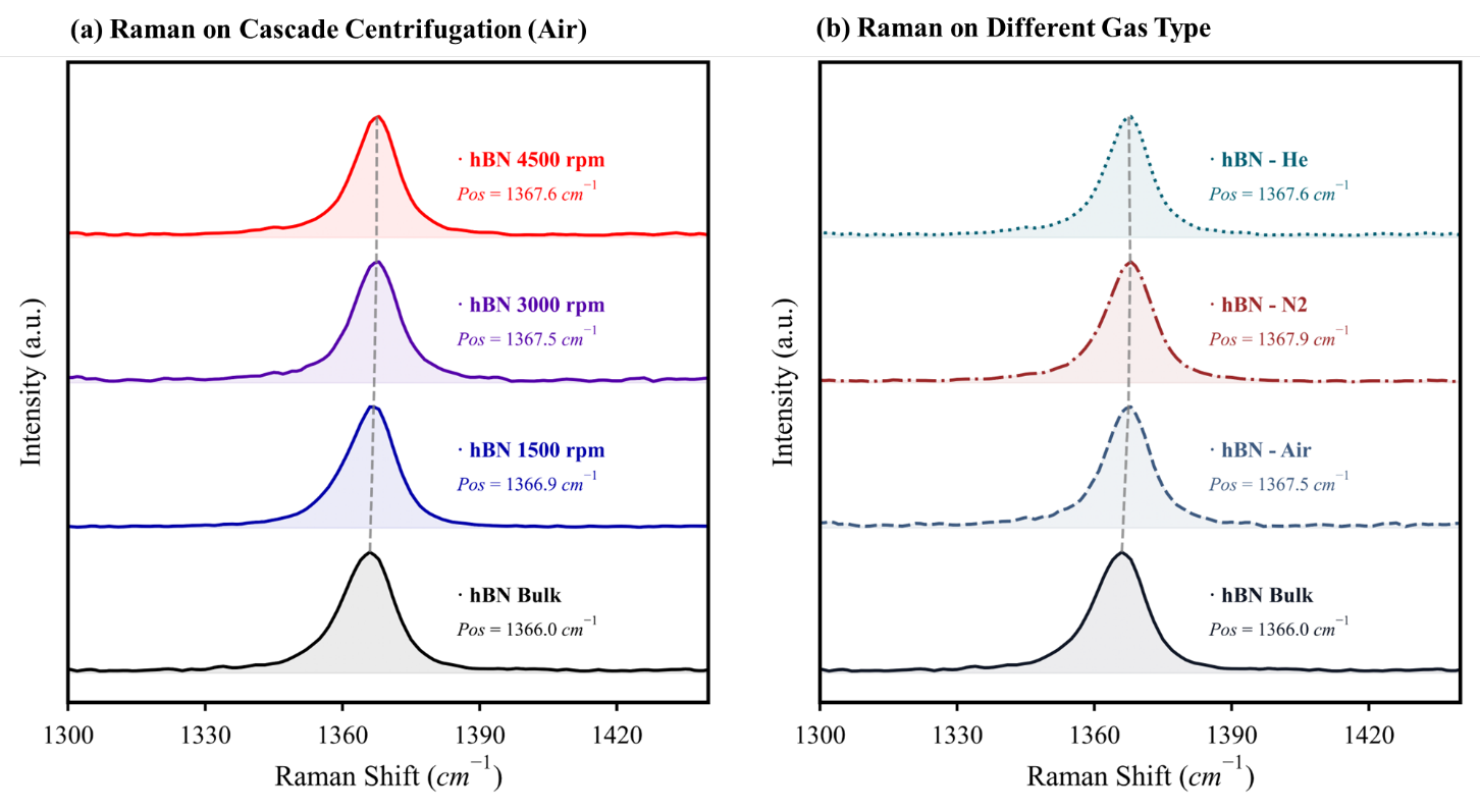
Graphene kept its characteristic G and 2D peaks—the named features in its Raman spectrum. Its D peak became stronger. That can happen when sheets have more exposed edges or more defects, so a stronger D peak alone does not prove damage inside the sheets.
The shape and relative strength of the graphene peaks were consistent with sheets containing several layers, rather than mostly single layers. h-BN also kept its characteristic vibrational peak.
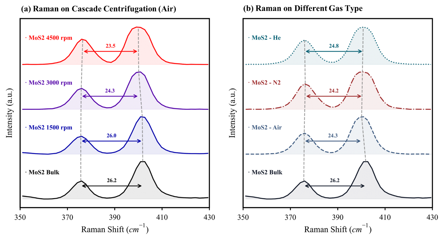
For MoS₂, I followed the gap between two peaks. That gap became smaller in the higher-speed centrifuge fractions shown below. Alongside the other measurements, this supported a greater share of thinner sheets. It did not give an exact layer count for every flake.
Go deeper: measurements and scientific details
The graphene 2D-band widths were approximately 73–79 cm⁻¹. Together with the reported peak-intensity ratios, they supported few-layer or multilayer graphene-rich sheets rather than a mainly single-layer product. The h-BN E₂g peak remained near 1366–1368 cm⁻¹.
For MoS₂, Δ = A₁g − E₂g¹ is the separation between an out-of-plane and an in-plane vibration, using the bulk-mode names in the thesis. In the air-processed series, the reported separation decreased from 26.21 cm⁻¹ for bulk material to 23.51 cm⁻¹ for the 4500 rpm fraction. The unit cm⁻¹ expresses Raman shift, a measure of the change in light energy.
The centrifuge separates the dispersion into fractions by spinning it. Here rpm means revolutions per minute and labels the experimental conditions. Speed alone is not a universal size or thickness cutoff: rotor radius, spinning time and liquid conditions also matter. Strain, electrical charge and temperature can also change Raman peaks, so peak separation alone does not give an exact layer count.
The instruments
UV–Vis spectrophotometer
How much solid is in the liquid?
Light of a selected wavelength passes through a small transparent cell called a cuvette. A detector measures how much gets through and compares it with the same liquid without flakes. The flakes absorb some light and scatter some away from the detector.
A graph of how strongly the sample reduces the detected light at different wavelengths. A calibration using known concentrations lets us estimate the concentration of an unknown sample.
More concentrated liquid often lets less light through, but flake size and clumping also change the reading. Compare similar samples within the calibrated range. A darker liquid does not automatically mean thinner sheets.
Used with gravimetric calibration in Chapter 6; MoS₂ spectral features also provided literature-calibrated size and thickness indicators.
TEM, STEM and HRTEM
Did we make sheets, and are atoms still locally ordered?
A beam of electrons passes through a very thin sample. In transmission electron microscopy (TEM), electromagnetic lenses form an enlarged image. Scanning transmission electron microscopy (STEM) scans a tightly focused beam across the sample, building the image point by point. High-resolution TEM (HRTEM) is a way of using TEM to see features linked to the repeating atomic structure.
Images that reveal flake shape, size, folds and edges. High-resolution images can also show repeating patterns in small regions of the crystal.
Only a small part of the batch reaches the microscope grid. Overlapping flakes, sample preparation and damage from the electron beam can affect the image. Brightness alone does not tell us an exact number of layers.
Chapter 7, Figures 7.1–7.4 and Table 7.1: morphology, local lattice preservation and representative dimensions.
Atomic force microscope (AFM)
How high is the flake above its support?
A very sharp tip on a flexible arm, called a cantilever, moves across the surface. A laser reflects off the arm onto a light sensor, revealing its motion. The instrument adjusts the vertical position to keep the tip–surface interaction steady, and uses those adjustments to build a height map.
A map of surface height. A line drawn across the map shows the step from the bare support to the top of a flake.
Water or residue under a flake can make it appear taller. The support and instrument settings matter too, and the tip can make narrow features look wider. Measured height needs careful checking before we turn it into a layer count.
Complementary method included to explain individual-flake height measurement; no original Chapter 7 AFM dataset is presented here.
Scanning electron microscope (SEM)
Are the flakes spread out or clumped together?
A narrow electron beam sweeps across the sample. It releases low-energy electrons from near the surface, called secondary electrons. A detector collects them, and the instrument builds an image from the signal at each beam position. Other detectors can collect electrons scattered back from the sample.
Images of surface features: particle shapes, clumps, gaps and how material covers a support.
The image does not directly count atomic layers or identify chemical bonds. Electrical charge can build up on insulating samples such as h-BN and distort the image. The electron beam and any coating added for imaging can also affect what we see.
Complementary technique explained for readers; the dissertation includes SEM in its literature discussion. My Chapter 7 morphology conclusions use TEM/STEM/HRTEM.
X-ray photoelectron spectrometer (XPS)
Has the surface chemistry changed?
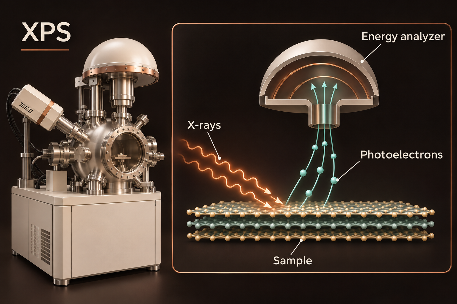
X-rays knock electrons out of the sample. The instrument measures the energy of those electrons to work out how tightly they were bound. Different elements and bonding environments leave different patterns of peaks in the resulting graph.
A spectrum: a graph showing how many electrons are detected at different energies. Its peaks help identify elements near the surface and the chemical states they are in.
Peaks can overlap, so separating them requires assumptions. Charge building up on the sample can shift their positions. Small amounts of a substance may go undetected, and handling or storage can change the surface before it is measured.
Chapter 7, Figures 7.5–7.14: retention of dominant bonding environments and moderate surface or edge modification.
Raman spectrometer
What do the atoms’ vibrations tell us?
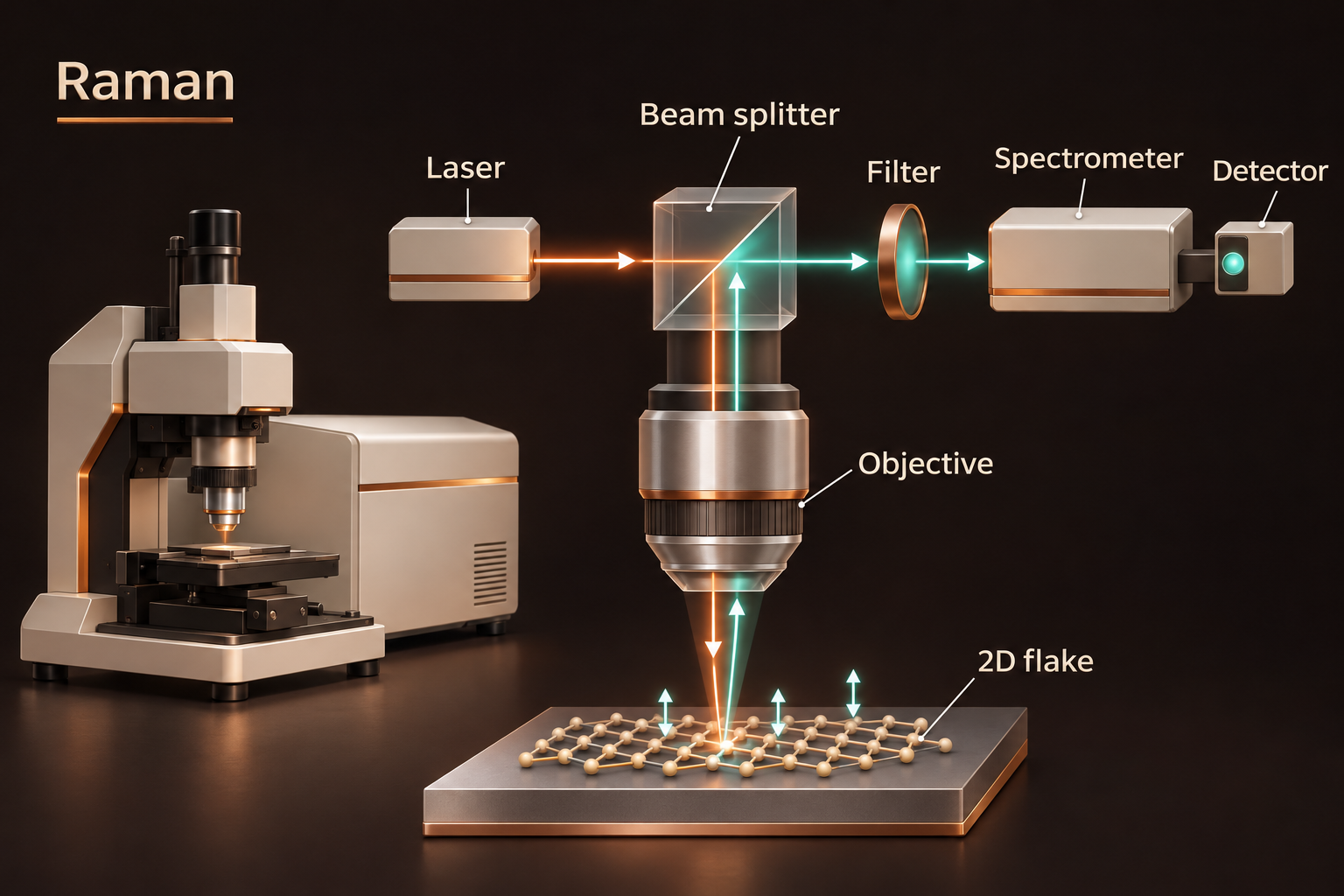
A laser shines on the sample. Most scattered light keeps the same energy, but a tiny fraction gains or loses energy through interactions with atomic vibrations. A filter removes the much stronger unchanged light, allowing the instrument to measure the small energy shifts.
A graph with peaks associated with different vibrations. The positions, widths and relative strengths of these peaks help us compare materials and detect changes.
Layer number is only one influence. Edges, defects, stretching of the crystal, electrical charge and heating by the laser can also change the peaks. We compare several features under similar conditions and check them against other measurements.
Chapter 7, Figures 7.15–7.17: graphene D/G/2D bands, the h-BN E₂g mode and MoS₂ mode separation.
Measured MoS₂ Raman peak separation
| Sample | Δ (cm⁻¹) |
|---|---|
| Bulk precursor | 26.21 |
| 1500 rpm fraction | 26.01 |
| 3000 rpm fraction | 24.28 |
| 4500 rpm fraction | 23.51 |
Lower separation supports thinner/few-layer enrichment; these are reported peak separations, not direct layer counts. Table 7.13 does not report measurement uncertainties.
Original thesis figures
Key takeaways
My measurements tell a connected story: the collected material contained sheets, their main bonding patterns remained, and their characteristic atomic vibrations were still present. For MoS₂, the Raman results also supported a greater share of thinner sheets in some fractions. This is evidence of successful exfoliation, but it does not mean every sheet has the same thickness or is free of defects. Understanding the whole batch would require measuring more flakes and combining more evidence.
Start with a question, then choose the instrument that can answer it.
Keep the illustration and the evidence separate: one explains the idea; the other shows what was measured.
Build a conclusion from several methods, and say clearly what the measurements leave uncertain.